The Fast Fourier Transform and its Quantum Analog

April 2, 2019

1   The Discrete Fourier Transform

The formula for the discrete fourier transform is as follows:
$$ X_k=\frac{1}{\sqrt{N}}\sum_{n=0}^{N-1}x_ne^{2\pi ikn/N} $$ What the heck is going on here? Without sufficient insight, this looks like a jumble of mysterious symbols. The goal of this section is to develop some intuition for what exactly the discrete Fourier transform does. A simple analogy that is both often used and quite helpful starts with considering the notes in a piece of music. The actual sound waves that make it to your ear are a ridiculously complex-looking function– to illustrate, take this sound bite.

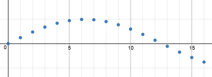
We can graph it as a function of pressure over time:

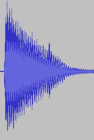
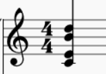
which looks dauntingly complicated. But listening to the sound itself, one would think that there's a simpler way to represent it: since it's just a single chord, we could write out the notes that make it up.

That's essentially all that the Fourier transform does! By converting between the time-domain and the frequency-domain, the Fourier transform can extract extremely valuable information out of an otherwise intangible signal.

Let's get back to that scary-looking equation. To begin, here's an overview (credit goes to Stuart Riffle) explaining what each symbol means:

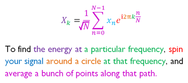
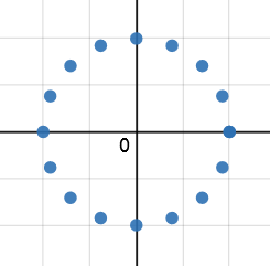
We start with a bunch of input data \(x_k\) where \(k\) ranges from 1 to \(N\), and by applying the discrete Fourier transform to that data we get as output \(X_k\). The central idea here is that weird looking exponential. It plays the role of winding, in a sense. Euler's formula tells us that $$ e^{i\varphi}=\cos(\varphi)+i\sin(\varphi) $$ Meaning that in the complex plane we can visualize the set of points \(e^{2\pi i n/N}\) for each \(n\in\{0,1,2,...,N-2,N-1\}\) as follows (in this example, arbitrarily taking N=16):

In the above equation for the DFT, though, you might notice that each point is multiplied by a scaling factor \(x_n\) based on the input data. For clarity, let's consider input data that appears to be periodic:

Wrapping this curve around a circle at various spacings and taking the average as we vary \(k\) can be visualized as follows:

To recap, we've seen that the discrete Fourier transform works by evenly twisting your input data around a circle and finding the "center of mass" for each possible arrangement. 3Blue1Brown has an extremely well-made video that presents the continuous Fourier transform this way, which you can find here. Another fantastic resource can be found here.

2   Speeding Things Up

In the previous section, we saw how the discrete Fourier transform can be thought of as a way to extract the frequency spectrum of an input by arranging your input data about a circle. In this section, we will explore the fast fourier transform (FFT), which is one of the most important algorithms of all time. The FFT significantly speeds up calculating the discrete Fourier transform by exploiting a certain periodicity in the computation. $$x= \left(\begin{matrix} x_1\\ x_2\\ \vdots\\ x_N \end{matrix}\right)\\$$ Recall that matrix multiplication works as follows: $$\text{If }X=Ax,\text{ then }X_i=\sum_jA_{ij}x_j$$ Let's introduce the shorthand \(\omega=e^{i2\pi/N}\). (Note that \(\omega^N=1\)) Going back to the formula from the previous section, we have $$X_n=\frac{1}{\sqrt{N}}\sum_{n=0}^{N-1}x_ne^{2\pi ikn/N}=\sum_{n=0}^{N-1}x_n\omega^{nk}$$ Hold on a second! We can write this sum as matrix multiplication. Consider the \(N\times N\) matrix \(F\) such that the entry \(F_{jk}=\omega^{jk}\). Let's write it out explicitly: $$F=\left(\begin{matrix} 1 & 1 & 1 & 1 & \dots & 1 & 1\\ 1 & \omega & \omega^2 & \omega^3 &\omega^4 & \dots & \omega^{N-1}\\ 1 & \omega^2 & \omega^4 &\omega^6 & \omega ^8 &\dots &\omega^{2(N-1)}\\ \vdots & & & & \ddots& & \vdots\\ 1 & \omega^{N-1} & \omega^{2(N-1)} & \omega^{3(N-1)} & \omega^{4(N-1)} & \dots & \omega^{(N-1)(N-1)} \end{matrix} \right)$$ So the discrete Fourier transform can be represented much more compactly as $$X=Fx.$$ You've probably noticed that the matrix \(F\) seems to have a lot of patterns going on inside it. The FFT essentially exploits these by shuffling the input data \(x\) a certain way so that the matrix multiplication can be recursively carried out on smaller matrices.

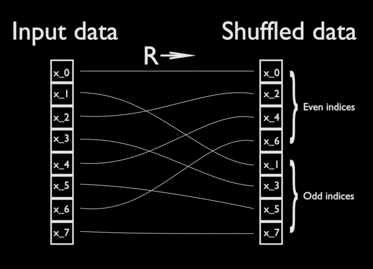
After shuffling the input by applying \(R\), one can verify that applying \(F\) to the original data is essentially equivalent to applying the DFT respectively to both the first half of the shuffled data and the second half. For the second (odd) half, we premultiply by a factor of \(\omega\). By splitting the matrix multiplication into only two calls of an \(N/2\times N/2\) matrix multiplication, followed by some linear-time arithmetic, the FFT gains significant speedup over the regular discrete Fourier transform: for a call to the FFT on an input of size \(N\), we have $$T(N)=2T(N/2)+O(N)$$ The master theorem tells us that this algorithm thus runs in time \(O(N\log N)\). If we take \(N=2^n\) to be the number of configurations of a bitstring of length \(n\), then we see that the FFT is order \(O\left(2^n\log(2^n)\right)=O(n2^n)\) in terms of the number of bits of input.

3   Using Quantum to Speed Things up Even More

The FFT gets its name for being fast. But is there an even better way to find the discrete Fourier transform? In 1994, Peter Shor (the genius behind Shor's Algorithm) provided us with an answer: yes! The quantum Fourier transform (QFT) exploits quantum weirdness to provide us with a way to compute the discrete Fourier transform in only \(O(n^2)\) time. In the previous section, we saw that the FFT runs in \(O(n2^n)\) time— this is an exponential speedup, and illustrates just how seriously powerful quantum computing can be. In the following analysis, we'll explain exactly how this speedup is possible. We'll be making relatively heavy use of linear algebra, which is (perhaps unfortunately) unavoidable in quantum computing. If you need a refresher on linear algebra, check out 3Blue1Brown's series here. Sheldon Axler's textbook Linear Algebra Done Right is also a fantastic resource.

The QFT is essentially the same transformation as the DFT, but now our input and output data are stored in quantum states, which we represent as kets (vectors). These kets live inside a Hilbert space, which is essentially just a vector space endowed with an inner product. Given an orthonormal basis \(\left| 0 \right>,\left| 1 \right>,\dots\left| N-1 \right>\), the QFT acts on one of the basis vectors \(\left| k \right>\) in essentially the same way as the DFT:

Discrete Fourier Transform: $$ X_k=\frac{1}{\sqrt{N}}\sum_{l=0}^{N-1}x_le^{2\pi ikl/N} $$ Quantum Fourier Transform: $$ QFT\left| k \right>=\frac{1}{\sqrt{N}}\sum_{l=0}^{N-1}\left| l \right>e^{2\pi ikl/N} $$

From here we can see that given an arbitrary input state \(\sum_{k=0}^{N-1}x_k\left| k \right>\), the QFT yields $$ \underbrace{\sum_{k=0}^{N-1}X_k\left| k \right>}_{\text{Output state}}= \sum_{k=0}^{N-1}\underbrace{\vphantom{\sum_{k=0}^{N-1}}X_k}_{\text{DFT on input amplitude $x_k$}}\left| k \right>=\sum_{k=0}^{N-1}\sum_{l=0}^{N-1}\frac{x_l}{\sqrt{N}}e^{2\pi ikl/N}\left| k \right> $$ Note that in a quantum computer, the dimension of the Hilbert space \(N\) must be a power of 2, since for each qubit in our quantum computer we multiply our state space by 2--- given \(n\) qubits, our state space has dimension \(N=2^n\). Hence we can rewrite the QFT's action on an input state as $$ QFT\left(\sum_{k=0}^{2^n-1}x_k\left| k \right>\right)=\sum_{k=0}^{2^n-1}\sum_{l=0}^{2^n-1}\frac{x_l}{\sqrt{2^n}}e^{2\pi ikl/2^n} $$ Because \(l\) ranges from 0 to \(2^n-1\), we can also represent it through its binary expansion: $$ l = \sum_{p=1}^{n}l_p2^{n-p} $$ Hence we can rewrite the QFT on a basis state \(\left| l \right>\) as $$ \begin{align*} QFT\left| k \right>&=\frac{1}{\sqrt{2^n}}\sum_{l=0}^{2^n-1}\left| l \right>\exp\left(2\pi ik \left(\sum_{p=1}^{n}l_p2^{n-p}\right)/2^{n}\right)\\ &=\frac{1}{\sqrt{2^n}}\sum_{l=0}^{2^n-1}\left| l \right>\exp\left(2\pi ik \left(\sum_{p=1}^{n}l_p2^{-p}\right)\right)\\ &=\sum_{l=0}^{2^n-1}\left| l \right>e^{2\pi ik l_1/2}\times e^{2\pi ik l_2/2^2}\times\dots\times e^{2\pi ik l_{n-1}/2^{n-1}}\times e^{2\pi ik l_{n}/2^{n}}\\ \end{align*} $$ Since each \(l_k\) is just a component of the binary expansion of \(l\), it can only take the values 0 or 1. Hence rather than summing over the \(2^n\) values of \(l\) ranging from 0 to \(2^{n-1}\), we can instead write \(\left| l \right>=\left|l_1l_2\dots l_{n-1}l_n\right>\) and sum over the \(2^n\) possible configurations of each \(l_i\): $$ \begin{align*} &=\frac{1}{\sqrt{2^n}}\sum_{l_1=0}^1\sum_{l_2=0}^1\dots\sum_{l_{n-1}=0}^1\sum_{l_n=0}^1\left|l_1l_2\dots l_{n-1}l_n\right>e^{2\pi ik l_1/2}\times e^{2\pi ik l_2/2^2}\times\dots\times e^{2\pi ik l_{n-1}/2^{n-1}}\times e^{2\pi ik l_{n}/2^{n}}\\ &=\frac{1}{\sqrt{2^n}}\sum_{l_1=0}^1\sum_{l_2=0}^1\dots\sum_{l_{n-1}=0}^1\sum_{l_n=0}^1\left|l_1\right>\otimes\left|l_2\right>\otimes\dots\otimes \left|l_{n-1}\right>\otimes\left|l_n\right>e^{2\pi i l_1/2}\times e^{2\pi i l_2/2^2}\times\dots\times e^{2\pi ik l_{n-1}/2^{n-1}}\times e^{2\pi ik l_{n}/2^{n}}\\ &=\frac{1}{\sqrt{2^n}}\sum_{l_1=0}^1\sum_{l_2=0}^1\dots\sum_{l_{n-1}=0}^1\sum_{l_n=0}^1e^{2\pi ik l_1/2}\left|l_1\right>\otimes e^{2\pi ik l_2/2^2}\left|l_2\right>\otimes\dots\otimes e^{2\pi ik l_{n-1}/2^{n-1}}\left|l_{n-1}\right>\otimes e^{2\pi ik l_n/2^n}\left|l_n\right> \end{align*} $$ Where from the first to second line we write out the tensor product of each state explicitly, and from lines two to three we rearrange scalar factors. From here, we can just write out the sum for each \(l_k\) explicitly: $$ =\frac{1}{\sqrt{2^n}} \left(\left|0\right>+e^{2\pi ik/2}\left|1\right>\right) \otimes \left(\left|0\right>e^{2\pi ik/2^2}\left|1\right>\right) \otimes \dots \otimes \left(\left|0\right>+e^{2\pi ik/2^{n-1}}\left|1\right>\right) \otimes \left(\left|0\right>+e^{2\pi ik/2^n}\left|1\right>\right) $$ We've shown then that on \(n\) qubits, the quantum Fourier transform superposes each qubit between the \(\left|0\right>\) and \(\left|1\right>\) state, where the \(\left|1\right>\) state picks up a phase depending on the input state. This results in a relatively straightforward implementation, which we'll draw using the standard quantum circuit notation:

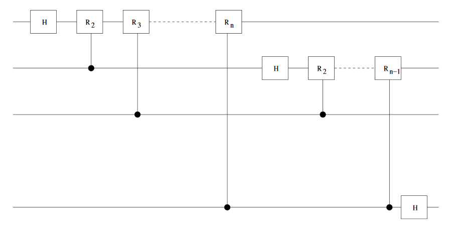
The most startling fact about this quantum analog to the classical discrete Fourier transform is the fact that only \(O(n^2)\) gates are required to implement it. Look at the diagram: you can see that we need \(n\) gates for the first qubit, plus \(n-1\) gates for the second, etc., adding up to a total of \(n(n+1)/2\) gates. Wheras the FFT scaled as \(O(n2^n)\), the QFT scales as \(O(n^2)\)— this is an exponential speedup over the fastest known classical means of calculating the discrete Fourier transform.

The QFT was developed by Peter Shor as part of his extremely famous factoring algorithm. If you'd like to look more into Shor's algorithm, check out here, or Rieffel and Polak page 163.